Interpreting Black Box Neural Networks to Improve Diabetic Retinopathy Diagnoses

Over the last few weeks, I've been looking at how neural networks trained to diagnose diabetic retinopathy are affected by the data they are trained on. By using interpretability methods on deep neural networks, we can identify unwanted correlations in the dataset, improve the network's predictions, enhance trust, and provide various explanations for predictions. Interpretation is not only useful to neural networks in general but vital to the applications that are particularly sensitive to the predictions - false negative diagnoses for a disease could lead to a patient's death and thus should be avoided when screening patients. In sensitive applications, like medical diagnostics, we want to be sure that the network has learnt relevant features for the particular disease in general and that it is identifying reasonable areas of the input for each particular case. Interpretability provides us with a toolkit to investigate neural networks for these desirable properties.

Diabetic Retinopathy

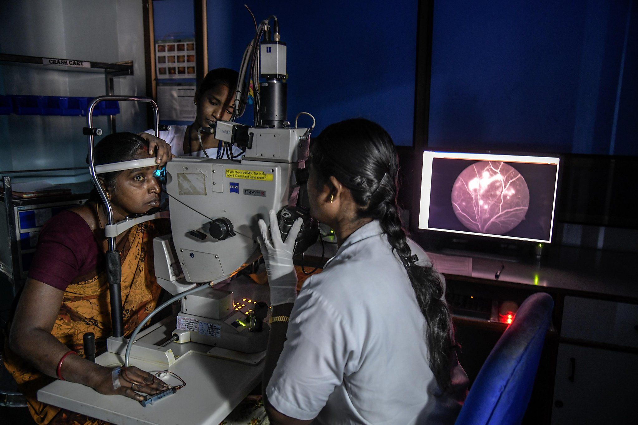
Here, I chose to apply interpretability to diabetic retinopathy (DR). DR is a disease of the retina that causes loss of vision. The disease typically occurs to people with a high blood sugar level. There are several symptoms to look for in the disease, where some of them are particularly subtle. If screened early enough, the disease can be reversed, however, if not, it can cause irreversible blindness. Therefore, it is vital that people in danger for the disease get screened regularly, however, there are often not enough doctors to look at every eye reliably. In work by Gulshan et al. [1], they noted that there was high variance across several doctors classifying images of retinas for DR. Even trained professionals can make mistakes in picking up the subtle signs of the disease. The image below outlines some of the pathologies related to diagnosing DR.

Using a neural network can help with picking up these symptoms and prevent loss of eyesight for many people. This is exactly what the work of Gulshan et al. and several others aimed to achieve [3,4]. However, ensuring that the network is, in fact, looking at features that are clinically relevant to a diagnosis is vital - if the network is picking up on other correlations in the dataset, then this could lead to a drop in model performance in the real world and, more importantly, result in false diagnoses for many people. Gulshan et al. [1] note this in their work:

Because the network “learned” the features that were most predictive for the referability [of DR] implicitly, it is possible that the algorithm is using features previously unknown to or ignored by humans. Although this study used images from a variety of clinical settings [...] the exact features being used are still unknown. Understanding what a deep neural net uses to make predictions is a very active area of research within the larger machine learning community.

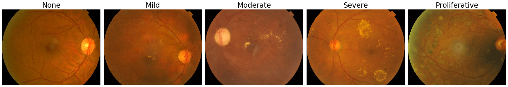
The dataset used is the 2019 APTOS Diabetic Retinopathy dataset [5]. This dataset contains 3662 retinal fundus images where each image is labelled from 0 to 4. Examples from the dataset are seen below. The networks that are trained are tested on a 20% subset of this dataset as well as on the IDRiD dataset [6]. The labels 0-4 correspond to no, mild, moderate, severe and proliferative DR.

Networks and Training

A ResNet34 [7] is used to make the predictions. The network is initialised from ImageNet [8] pretrained weights and the last BatchNorm and Linear layers are replaced with a custom head. The custom head is a sequence of adaptive pooling, BatchNorm, dropout, and Linear layers. All of the networks are trained in the same way with the same learning rates. The networks are trained for 38 epochs with reducing learning rates over time. The networks are trained with a one cycle schedule [9, 10] with cosine annealing [11]. With the 21 million learnable parameters in the ResNet34, it is not obvious how the network comes to its diagnoses of DR. In comes interpretability.

Interpretability

Interpreting deep neural networks is done in several ways, however, here I focus on methods that can be applied to many neural networks in general. These methods are the model-free methods discussed in the last post: visualisation and attribution. Visualisation methods generate an input that will highly activate a particular feature of the network, allowing us to see what the network is looking for [12]. We can generate inputs that target entire layers, channels or single neurons. Attribution tells us the parts of the input that are important in making the prediction of a particular class. The exact attribution method used is Grad-CAM [13] where the convolutional feature maps are weighted by the gradient.

A general method for applying interpretability is outlined below. This method is used on our ResNet.

1. Train a network on the dataset.
2. Apply attribution and visualisation methods to the trained network to identify data leaks and areas where the model can be improved. Adjust the dataset and model in line with these findings. Plot the inputs that result in the greatest losses in order to see what may be going wrong. Plot the confusion matrix to verify some of these claims.
3. Retrain the network using these fixes.
4. Reapply the same interpretability methods, ensuring that the network is now functioning the way that is desired. Repeat 3 and 4 as necessary.
5. Once the trained model is evaluated on the hidden test set, final interpretations can be done to validate a level of trust in predictions. Visualisations can indicate what features the model has learned in a visual way. Attribution can show what the network finds important when looking at examples from the dataset.

Baseline Network

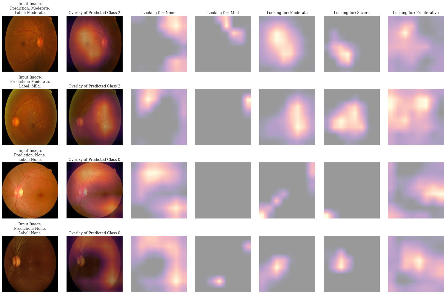
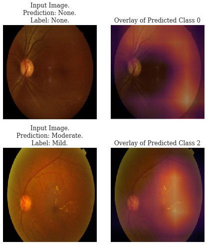
The first network, trained as outlined above, is our baseline. We apply Grad-CAM attribution to several predictions to identify patterns in the predictions. Two examples of the attribution maps are shown below. The attributions show worrying behaviour. First, the network attends to the black background of images labelled as "None" instead of at the retina, indicating a data leak. The data has an unwanted correlation where there is far more black background in the images that have no DR. Additionally, the network often predicts class 2 instead of 3 or 4 despite looking at the correct areas in the attribution. Our dataset is skewed and the network has not extracted enough signal to differentiate the minority classes.

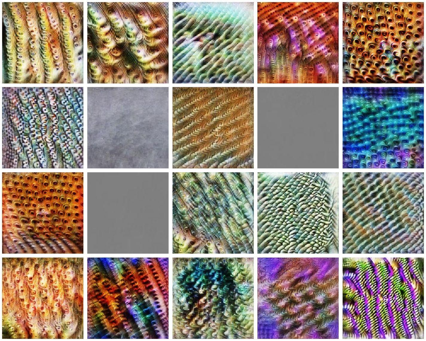
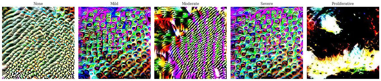
We also apply feature visualisation to the network. The class visualisations show similarly poor parameterisation. While class 0 and 2 seem to have learnt something, the features aren't clear. Additionally, class 1 and 3 have very similar visualisations indicating that the network can't tell them apart, thinking that they have the same features. Finally class 4 is completely under-parameterised, with barely any signal to create a cohesive visualisation.

Improved Network

After observing these issues in our network, we adjust the dataset. The combat the black background data leak, all of the images are processed to remove as much of the black background as possible. Additionally, we add a suite of augmentations to the dataset. Each image sampled from the dataset is randomly rotated, scaled, shifted, or adjusted in contrast, brightness and saturation. These augmentations will help prevent overfitting to the dataset but, perhaps more importantly, introduce more signal into the training process. The improved network should be invariant under these transformations - the network should extract features relevant to the set of transformed images (a larger, more diverse set) rather than the just the original images. These augmentations should help address the data imbalance by providing additional signal. The scale augmentations should also help avoid the data leak.

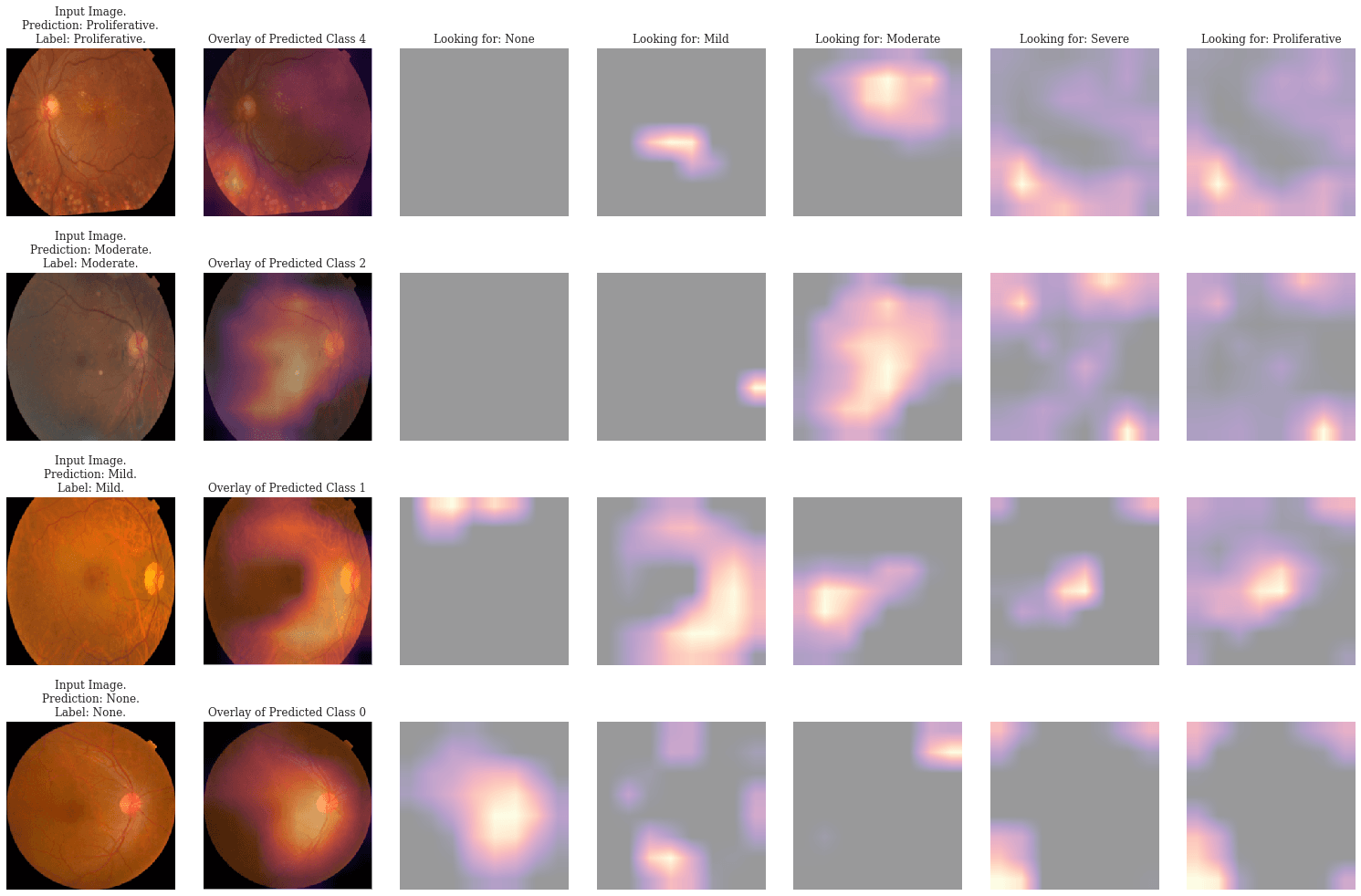
The network is retrained and the attribution maps of the network are redone. The network not only has a higher accuracy but more importantly, we can see from the Grad-CAM attributions that the network attends to the body of the retina when the predicted class is 0. Additionally, the minority classes are better represented, with fewer misclassifications seen in class 2.

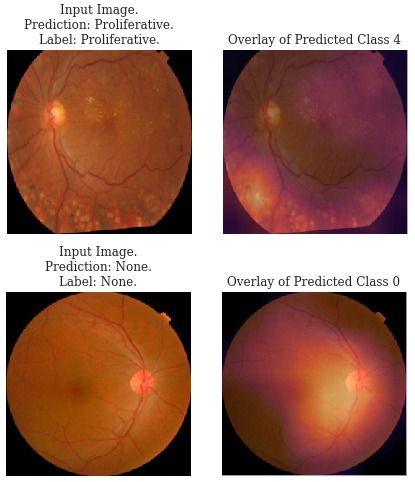
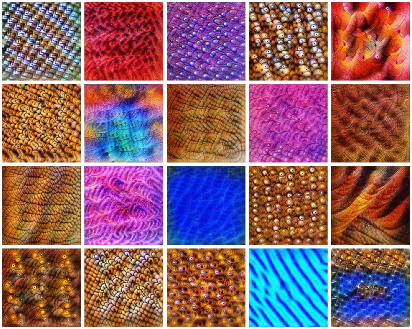
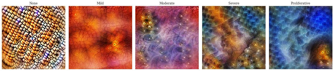
The class visualisations are also much better. The classes of DR show a visible progression in the amount of the disease present. In class 1 there are only a few small hard exudates which increase up to class 3. Class 4 has a large cohesive block of hard exudates and the green-blue hue that seems to be often present in the images of proliferative DR. Class 0 seems to be looking for general colours of healthy retinas - a mix of orange and white. This visualisation is far more encouraging that the network has learnt relevant features. With these improved interpretations we can better trust that the network is doing what we want it to without acting on extraneous information.

Overall results

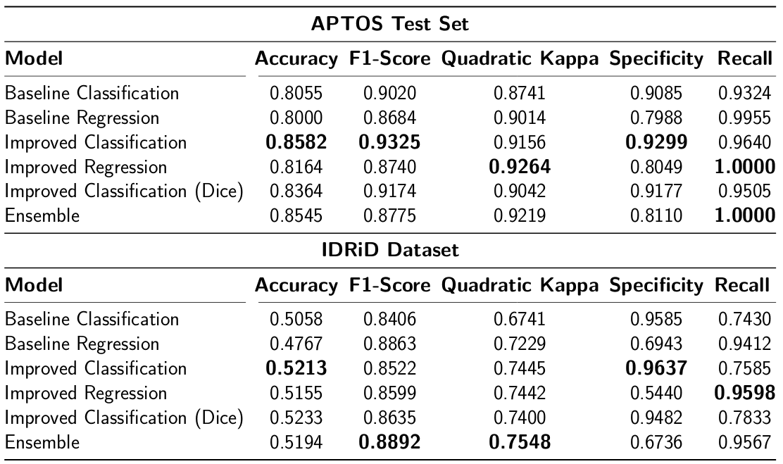
On top of the improvements observed in the interpretations, we see quantitative improvements in the performance of the networks across a variety of metrics. Furthermore, instead of just classifying the outputs, we change the model to regression, which is better suited to the task. An additional classification model is trained using Dice loss in an attempt at better optimising the F-score of the network. Finally, an ensemble of the improved classification, regression and Dice classification is created by averaging the predictions. The networks are also tested on the IDRiD dataset. This dataset represents an out of distribution test and indicates the generalisation of the networks. The metrics that apply to binary classifications (F1-score, recall, specificity) use "referable" DR as the classifier. This is defined as having greater than or equal to moderate DR [1].

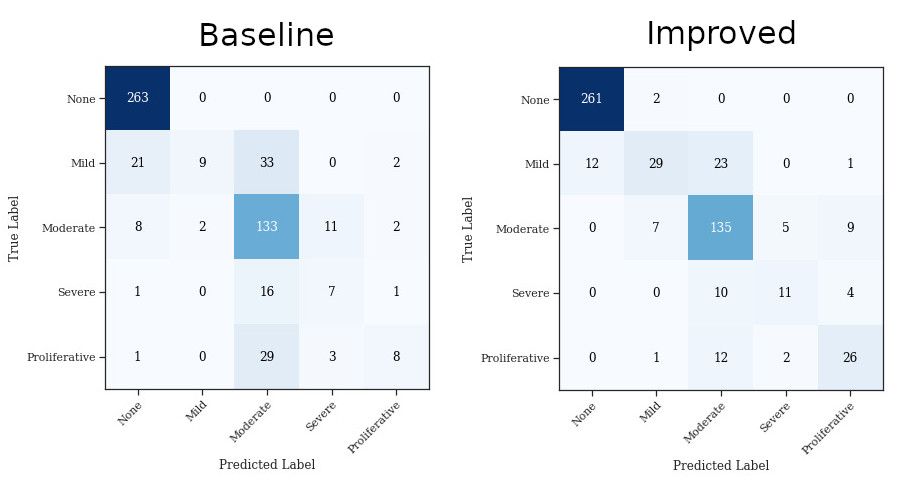
The confusion matrices of both baseline and improved networks are plotted alongside. The baseline network confusion matrix indicates the skewness of the classes while the improved network confusion matrix shows better overall performance across classes.

Conclusions

By interpreting the networks, we are able to improve performance and ensure that predictions are based on reasonable features. This enables trust in the network better supporting end users in identifying what the network has learnt. The key take-aways are:

1. Interpretability can help improve deep neural networks.
2. Data leaks and unwanted model shortcuts can be identified and prevented.
3. Models can be better trusted through explanations.
4. Visualisation show the features the network has learnt.
5. Attribution helps identify key areas of the dataset while training.

There is still much to be done in understanding and interpreting deep neural networks. Below, I outline avenues which would be particularly useful in furthering the work done here.

1. Develop a metric for relative importance across layers of the network to aide interpretations.
2. Improve the interface to interpretability methods by intelligent use of human-computer interface design.
3. Determine the effect of different loss functions on interpretations.
4. Standardize the testing of interpretability methods through quantitative measures and standard datasets.

References

[1] V. Gulshan et al., "Development and validation of a deep learning algorithm for detection of diabetic retinopathy in retinal fundus photographs," JAMA, 2016.

[2] Ophthalmology Physicians and Surgeons, "Treating diabetic retinopathy." 2019.

[3] J. Krause et al., "Grader variability and the importance of reference standards for evaluating machine learning models for diabetic retinopathy," Ophthalmology, vol. 125, no. 8, pp. 1264--1272, Aug. 2018.

[4] R. Sayres et al., "Using a deep learning algorithm and integrated gradients explanation to assist grading for diabetic retinopathy," Ophthalmology, vol. 126, no. 4, pp. 552--564, Apr. 2019.

[5] APTOS, "APTOS 2019 blindness detection." 2019.

[6] P. Porwal et al., "Indian diabetic retinopathy image dataset (idrid)." IEEE Dataport, 2018.

[7] K. He, X. Zhang, S. Ren, and J. Sun, "Deep residual learning for image recognition," CoRR, vol. abs/1512.03385, 2015.

[8] O. Russakovsky et al., "ImageNet Large Scale Visual Recognition Challenge," International Journal of Computer Vision (IJCV), vol. 115, no. 3, pp. 211--252, 2015.

[9] L. N. Smith, "A disciplined approach to neural network hyper-parameters: Part 1 - learning rate, batch size, momentum, and weight decay," CoRR, vol. abs/1803.09820, 2018.

[10] I. Loshchilov and F. Hutter, "SGDR: stochastic gradient descent with restarts," CoRR, vol. abs/1608.03983, 2016.

[11] J. Howard, "Now anyone can train imagenet in 18 minutes." 2018.

[12] C. Olah, A. Mordvintsev, and L. Schubert, "Feature visualization," Distill, 2017.

[13] R. R. Selvaraju, A. Das, R. Vedantam, M. Cogswell, D. Parikh, and D. Batra, "Grad-cam: Why did you say that? Visual explanations from deep networks via gradient-based localization," CoRR, vol. abs/1610.02391, 2016.

Appendix

The code that was used to generate all of the interpretations is made available here: https://github.com/ttumiel/interpret