Annotated LLaMA-3 Language Model

The LLaMA language models are powerful open-source foundation models by Meta's AI research team spanning 8-400 billion parameters. They're simple to understand and perform well, but best of all the entire model can be implemented in only 300 lines of code.

In this post we'll look at the architecture from a high level, as well as Meta's PyTorch code implementation, and hopefully some understanding of the different operations along the way. I include both the code as the "ground truth" implementation plus some 2D visualizations to help get a feel for the numbers. While the math is accurate, and identical to a transformer with an embedding dimension of 2, keep in mind that some interesting things happen in high dimensions that may seem unintuitive.

LLaMA 3 Architecture

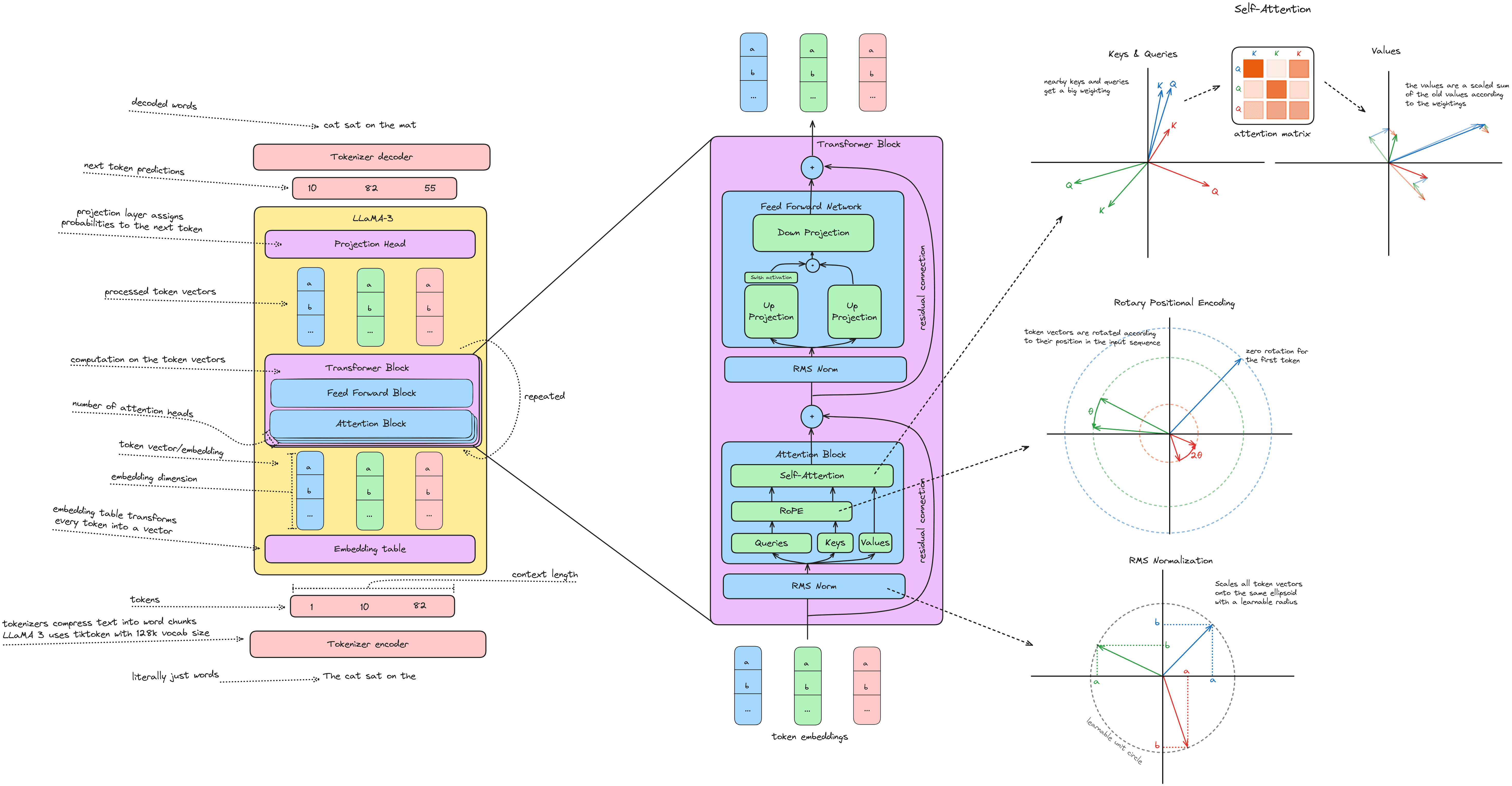
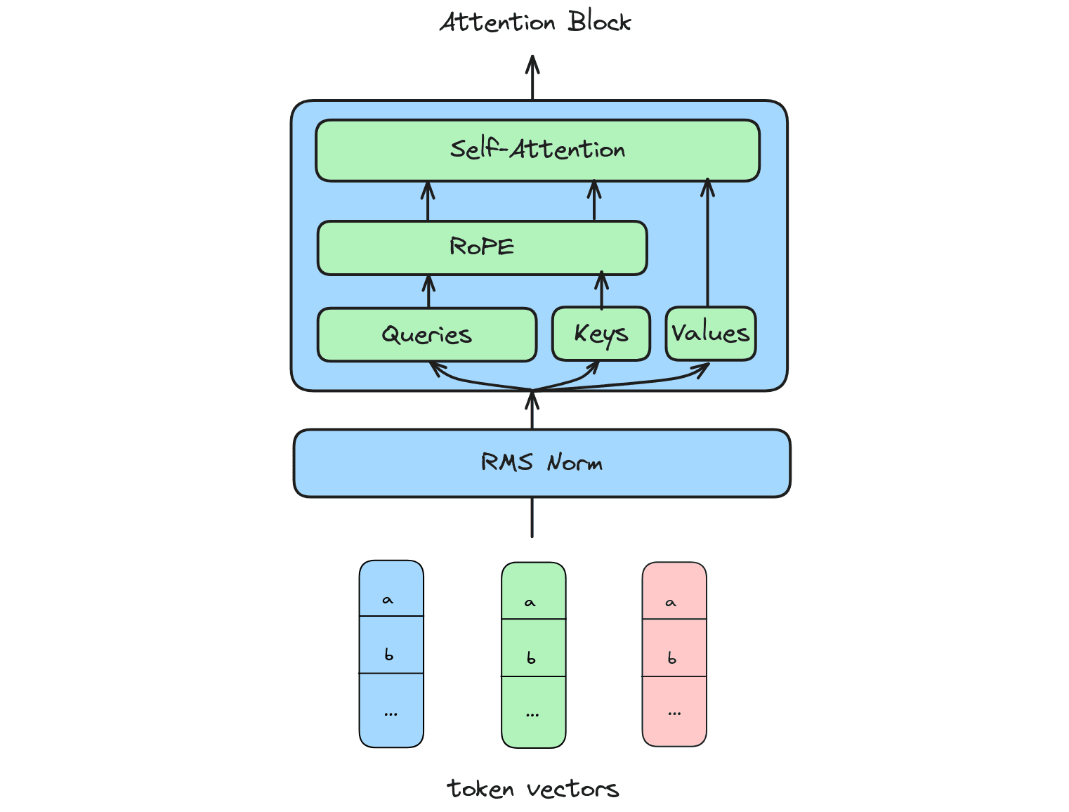
LLaMA 3 is a standard dense attention transformer, with a few small tricks packed in. Instead of layer norm, it uses RMS norm; instead of absolute postional encodings, it uses rotary positional encodings (RoPE); and it uses grouped query attention instead of multi-head attention.

Feel free to refer back to the architecture diagram above for any terminology that isn't familiar.

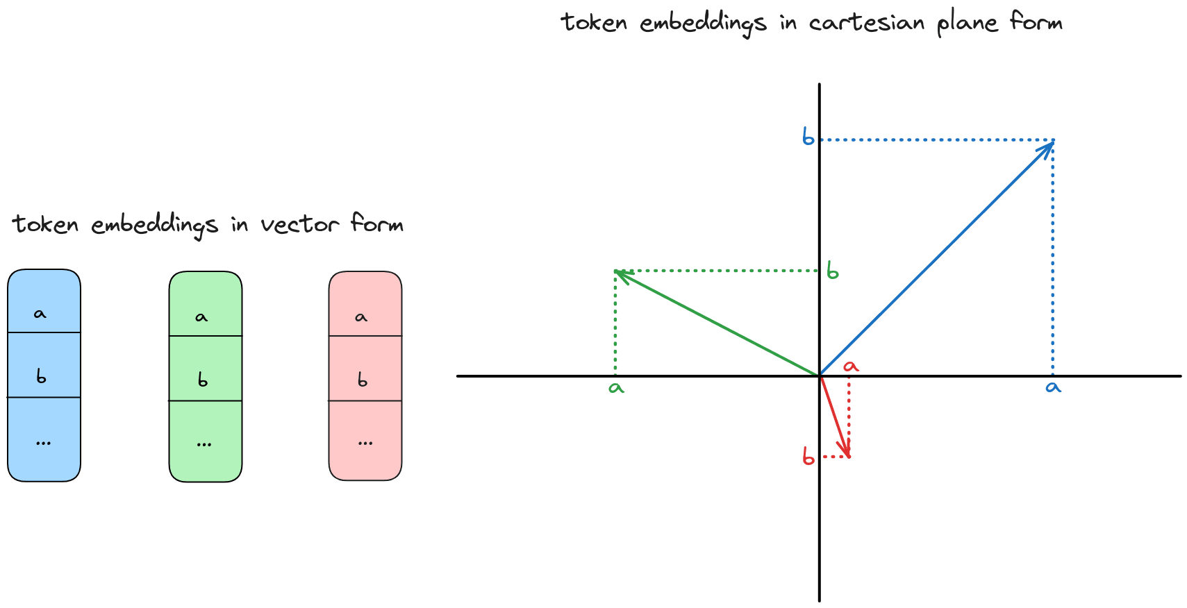
Each token vector is a series of numbers. I display these as small vector blocks and I also plot them in 2D as arrows on a cartesian plane. The arrows should give some intuitions, but not all low dimensional intuitions map well to high dimensions.

For a more detailed introduction to the transformer, and attention in general, check out The Illustrated Transformer.

RMS normalization

RMS normalization standardizes the $L^2$ norm of every token vector so that they all have a Euclidean length of 1. It also allows the network to learn to change the set length over time, turning the unit circle into an ellipse.

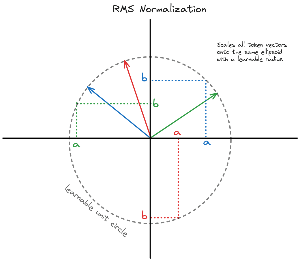
Normalization is vital for training large neural nets, and while layernorm has been most popular in language modelling, RMS norm has come up as a simpler, faster alternative because it doesn't need to calculate the mean and standard deviation of every vector. Previously I wrote about the importance of gradient scaling using different normalization methods - RMS norm does the same, just at reduced computational cost.

In math notation, it looks like this, where $x$ is a token vector and $W$ is the learnable weight.

RMS norm implementation

The code is a simple pytorch module that divides token vectors x by the $L^2$ norm of x, making sure to broadcast over all the values in the vector. We also have an epsilon argument to prevent numerical instability.

class RMSNorm(torch.nn.Module):
    def __init__(self, dim: int, eps: float = 1e-6):
        super().__init__()
        self.eps = eps
        self.weight = nn.Parameter(torch.ones(dim))

    def forward(self, x):
        output = x * torch.rsqrt(x.pow(2).mean(-1, keepdim=True) + self.eps)
        return output * self.weight

Rotary positional encoding

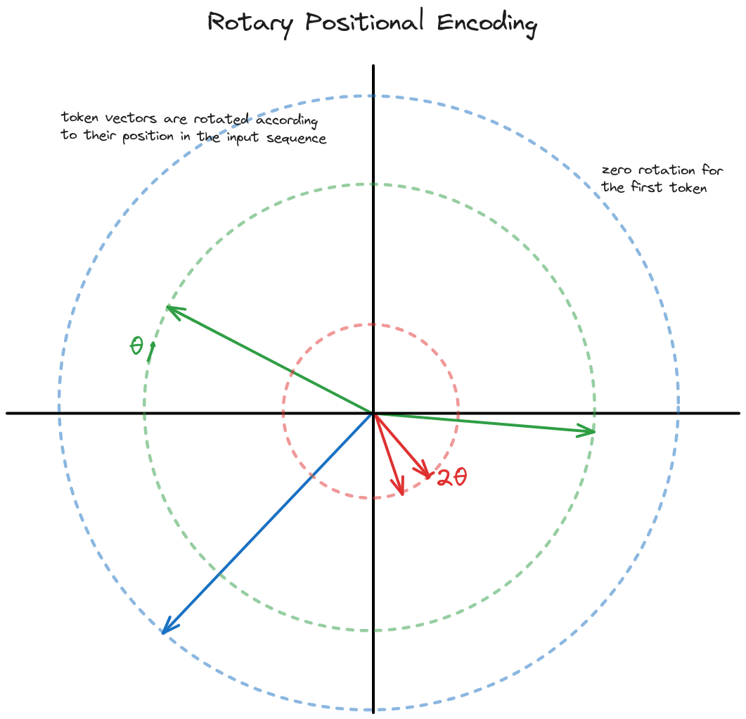
Rotary positional encoding (RoPE) is a parameter-free technique to encode positional information into the permutation-invariant self-attention operation by rotating token vectors.

That's a mouthful! Basically, every token vector is rotated around a circle by $p\theta$. So the first token is rotated by $\theta$, the second by $2\theta$, and so on. As a result, we can tell where each token is relative to the others, enabling us to learn positional relationships in language.

RoPE is applied to the query and key matrices inside the attention block, meaning they directly influence the attention scores in the attention calculation, but then they disappear. As a result, all of the attention blocks have RoPE included.

RoPE also comes with some nice bonuses:

• Token distances are preserved across positions - 3 tokens apart is always $3\theta$ apart. Distances are stable with RoPE.
• The rotations are constructed so that closer positions have a higher dot product. Intuitively, closer tokens have more to do with each other - but this can be unlearnt.
• The keys can be cached better than relative positions since a token's rotation is static, and doesn't depend on subsequent words.
• RoPE is a similarity transformation on the attention matrix.
  Sidenote You remember your linear algebra? The similarity transform is what gives us most of these nice properties - RoPE is constructed as an orthogonal matrix, so the transpose is the inverse!

Scaling context length with RoPE

Also, RoPE scales to long context lengths in a straightforward way, allowing longer contexts without much fuss, although you do need to set the period of the rotation carefully. A bigger base value gives more unique rotations (think "available positions"), but you should also train on those unique rotations with a long context length. Smaller base values (much smaller than the context length) seem to work equally well though and don't require training on long contexts as much.

LLaMA 3.1 slowly increases the original 8K context length model up to 128K during pre-training by increasing the base frequencies incrementally.

RoPE code implementation

First we can precompute and store the rotational frequencies. Every 2 embedding values in RoPE get a different rotational frequency scaled by the base value.

def precompute_freqs_cis(dim: int, end: int, base: float = 10000.0):
    # Calculate rotation frequencies using the embedding dimension and base value
    # theta_i = base^{-2i/d} for i in [0, dim//2)
    freqs = 1.0 / (base ** (torch.arange(0, dim, 2).float() / dim))

    # Generate the rotations for every position using the freqs
    t = torch.arange(end, device=freqs.device, dtype=torch.float32)
    freqs = torch.outer(t, freqs)

    # Convert the rotations to complex numbers (polar form) with magnitude 1
    freqs_cis = torch.polar(torch.ones_like(freqs), freqs)
    return freqs_cis

Then inside the attention block, we apply the rotation to the keys and queries using the pre-calculated frequencies.

def apply_rotary_emb(
    xq: torch.Tensor,  # (B, context_len, heads, dim)
    xk: torch.Tensor,  # (B, context_len, heads, dim)
    freqs_cis: torch.Tensor,  # (context_len, dim // 2)
) -> Tuple[torch.Tensor, torch.Tensor]:
    # Group the keys and queries into twos and view them as complex numbers
    xq_ = torch.view_as_complex(xq.float().reshape(*xq.shape[:-1], -1, 2))
    xk_ = torch.view_as_complex(xk.float().reshape(*xk.shape[:-1], -1, 2))

    # Prepare the frequencies to broadcast by unsqueezing the batch dim
    freqs_cis = reshape_for_broadcast(freqs_cis, xq_)

    # Rotate the keys and queries in the complex domain
    xq_out = torch.view_as_real(xq_ * freqs_cis).flatten(3)
    xk_out = torch.view_as_real(xk_ * freqs_cis).flatten(3)
    return xq_out.type_as(xq), xk_out.type_as(xk)

This video goes more into the history of absolute and relative positional encodings and how they related to RoPE.

Grouped Query Attention

LLaMA-3 uses grouped query attention (GQA) instead of multi-head attention (MHA). This reduces the number of heads in the key and value attention matrices to increase training speed and reduce memory consumption.

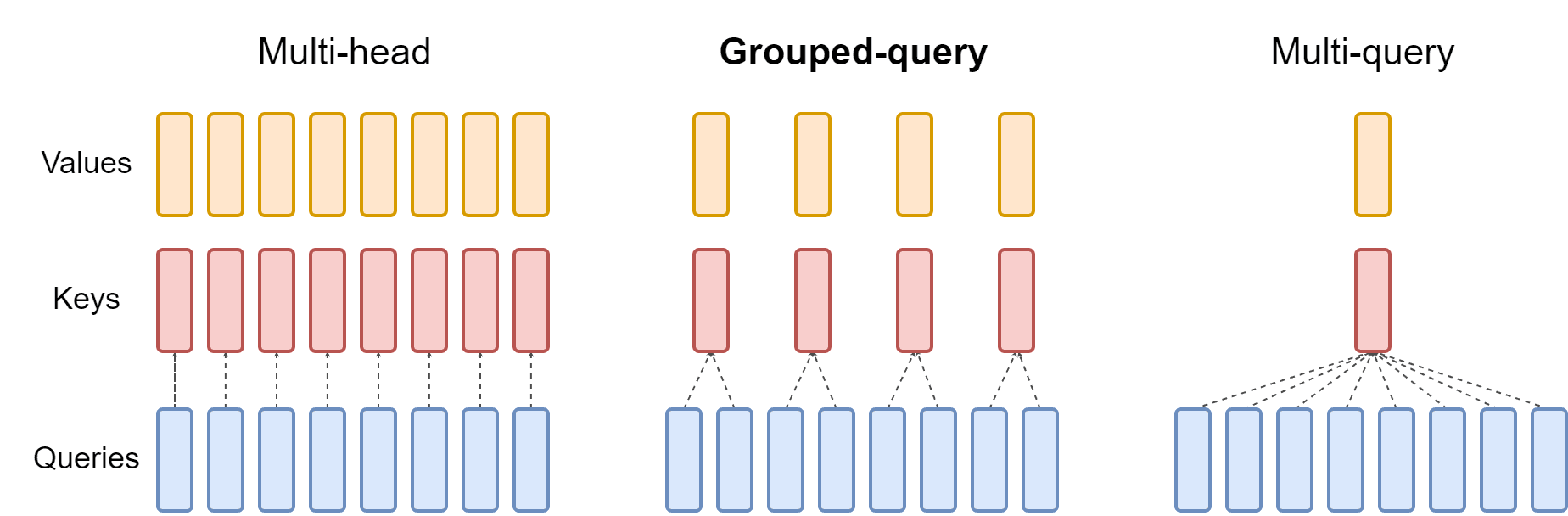
First we setup the GQA module with smaller key and query layers so that for every key and query head we have multiple value heads (4 for LLaMA 8B, 8 for 70B, 16 for 405B). Then we transform the token embeddings into the keys, queries and values and reshape them into their individual heads.

# Generate QKV matrices
queries, keys, values = self.wq(x), self.wk(x), self.wv(x)

# Reshape into number of heads for each
queries = queries.view(bsz, seqlen, self.n_heads, self.head_dim)
keys = keys.view(bsz, seqlen, self.n_kv_heads, self.head_dim)
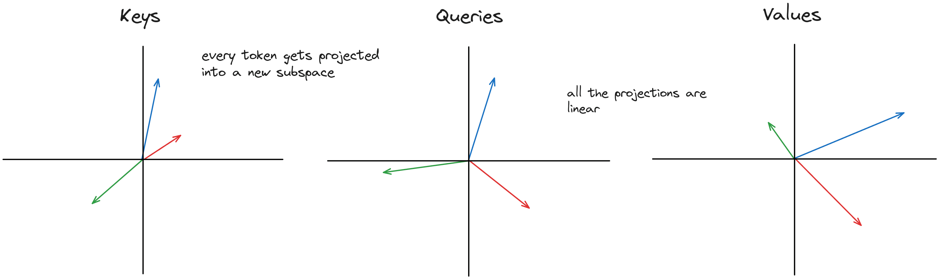
values = values.view(bsz, seqlen, self.n_kv_heads, self.head_dim)

The Q, K, V transform is the same for every vector so all token vectors are transformed by the same matrix. One linear transform for every head in each Q, K and V matrix that projects the embeddings into key, query and value-space.

Then we rotate the keys and queries with RoPE, preserving vector magnitudes.

# Apply RoPE
queries, keys = apply_rotary_emb(queries, keys, freqs_cis=freqs_cis)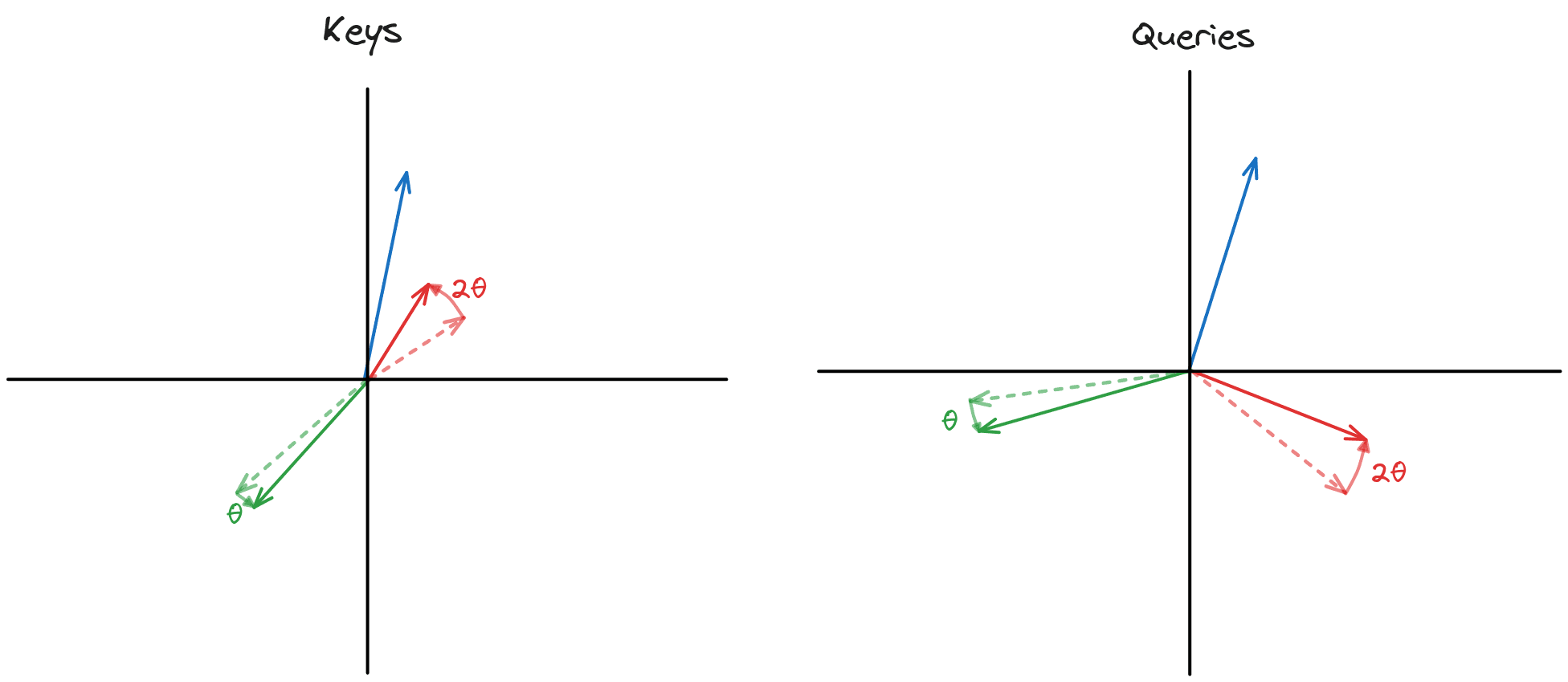

Then we repeat the keys and values so that they are applied as groups to the queries.

# repeat k/v heads if n_kv_heads < n_heads
keys = repeat_kv(keys, self.n_repeats)  # (bs, cache_len + seqlen, n_heads, head_dim)
values = repeat_kv(values, self.n_repeats)  # (bs, cache_len + seqlen, n_heads, head_dim)

And then the rest of the attention calculation proceeds as per usual: if the Q and K vectors are close, the dot product is large, increasing the weight in the attention matrix. The values are combined using the softmax probabilities in a weighted sum into the new values for each token vector.

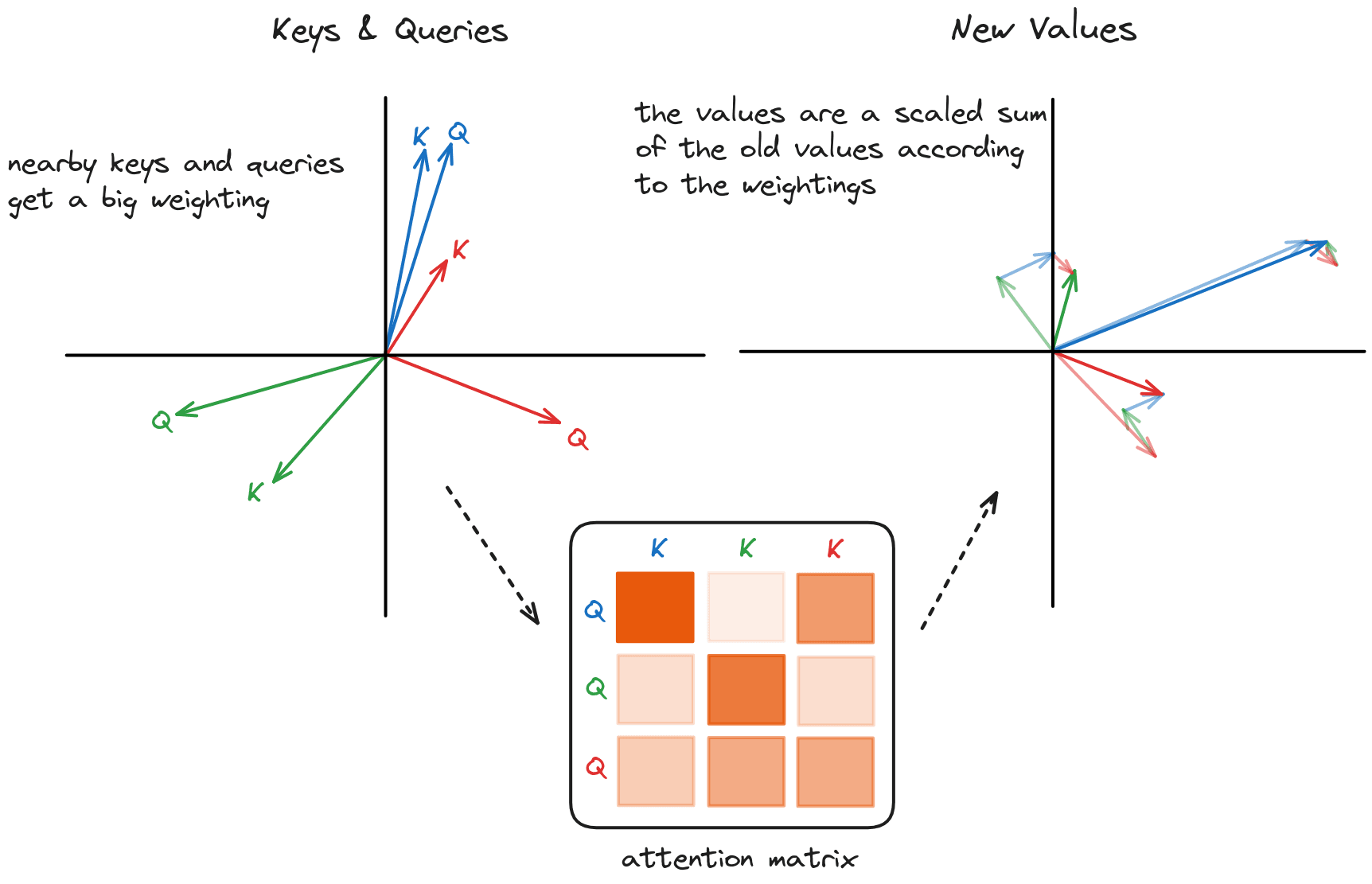
So that's what our attention block looks like!

Here's the full GQA implementation:

class GroupedQueryAttention(nn.Module):
    def __init__(self, args: ModelArgs):
        super().__init__()
        self.n_kv_heads = args.n_heads if args.n_kv_heads is None else args.n_kv_heads
        self.n_heads = args.n_heads
        self.n_repeats = self.n_heads // self.n_kv_heads
        self.head_dim = args.dim // args.n_heads

        self.wq = nn.Linear(
            args.dim,
            args.n_heads * self.head_dim,
            bias=False,
        )
        self.wk =  nn.Linear(
            args.dim,
            self.n_kv_heads * self.head_dim,
            bias=False,
        )
        self.wv =  nn.Linear(
            args.dim,
            self.n_kv_heads * self.head_dim,
            bias=False,
        )
        self.wo =  nn.Linear(
            args.n_heads * self.head_dim,
            args.dim,
            bias=False,
        )

    def forward(
        self,
        x: torch.Tensor,
        start_pos: int,
        freqs_cis: torch.Tensor,
        mask: Optional[torch.Tensor],
    ):
        bsz, seqlen, _ = x.shape

        # Generate QKV matrices
        queries, keys, values = self.wq(x), self.wk(x), self.wv(x)

        # Reshape into number of heads for each
        queries = queries.view(bsz, seqlen, self.n_heads, self.head_dim)
        keys = keys.view(bsz, seqlen, self.n_kv_heads, self.head_dim)
        values = values.view(bsz, seqlen, self.n_kv_heads, self.head_dim)

        # Apply RoPE
        queries, keys = apply_rotary_emb(queries, keys, freqs_cis=freqs_cis)

        # repeat k/v heads if n_kv_heads < n_heads
        keys = repeat_kv(keys, self.n_repeats)  # (bs, cache_len + seqlen, n_heads, head_dim)
        values = repeat_kv(values, self.n_repeats)  # (bs, cache_len + seqlen, n_heads, head_dim)

        queries = queries.transpose(1, 2)  # (bs, n_heads, seqlen, head_dim)
        keys = keys.transpose(1, 2)  # (bs, n_heads, cache_len + seqlen, head_dim)
        values = values.transpose(1, 2)  # (bs, n_heads, cache_len + seqlen, head_dim)

        # Calculate self-attention matrix
        scores = torch.matmul(queries, keys.transpose(2, 3)) / math.sqrt(self.head_dim)
        if mask is not None:
            scores = scores + mask  # (bs, n_heads, seqlen, cache_len + seqlen)
        scores = F.softmax(scores.float(), dim=-1).type_as(queries)

        # Get the output
        output = torch.matmul(scores, values)  # (bs, n_heads, seqlen, head_dim)
        output = output.transpose(1, 2).contiguous().view(bsz, seqlen, -1)
        return self.wo(output)

Feedforward network

LLaMA-3 also has a simple feedforward network which does computation independently on each token vector.

In fact, this little block is it's own neural network within the larger transformer. For an excellent analysis of it's operation you should read Chris Olah's Neural Networks, Manifolds, and Topology blog.

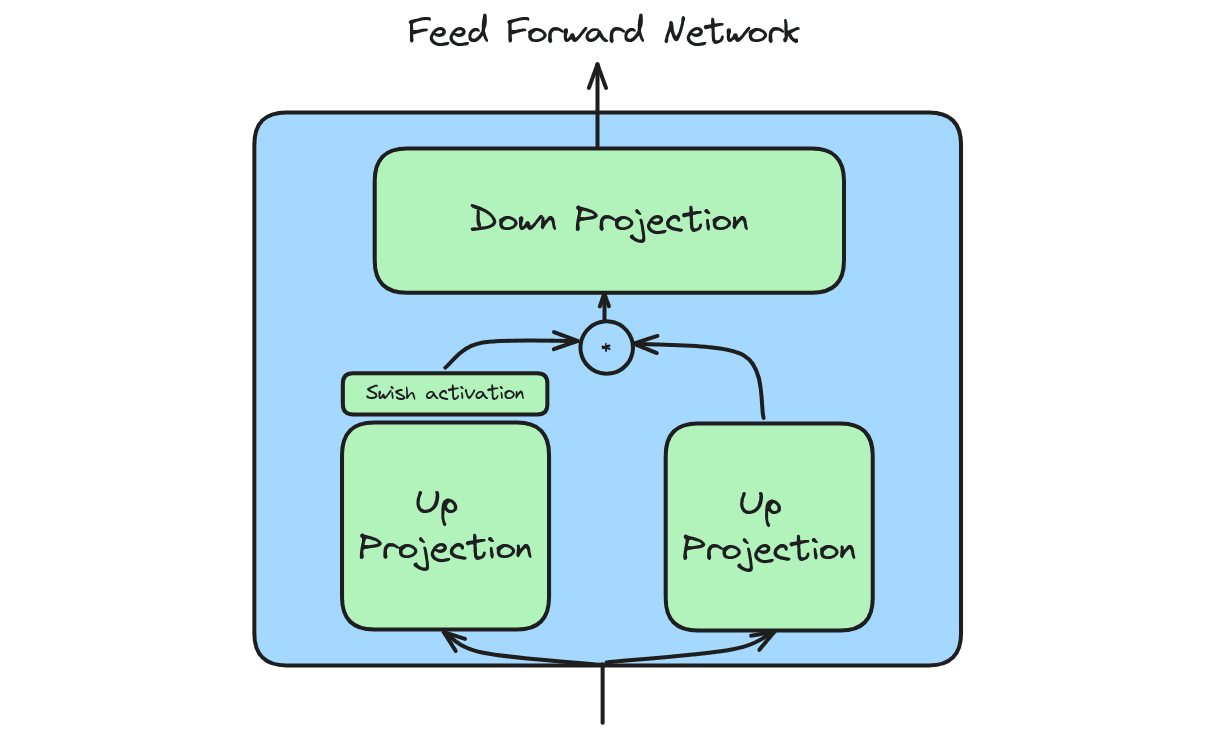
The code follows the architecture diagram quite similarly.

class FeedForward(nn.Module):
    def __init__(
        self,
        dim: int,
        hidden_dim: int,
        multiple_of: int,
        ffn_dim_multiplier: Optional[float],
    ):
        super().__init__()
        hidden_dim = int(2 * hidden_dim / 3)
        # custom dim factor multiplier
        if ffn_dim_multiplier is not None:
            hidden_dim = int(ffn_dim_multiplier * hidden_dim)
        hidden_dim = multiple_of * ((hidden_dim + multiple_of - 1) // multiple_of)

        self.w1 = nn.Linear(dim, hidden_dim, bias=False)
        self.w2 = nn.Linear(hidden_dim, dim, bias=False)
        self.w3 = nn.Linear(dim, hidden_dim, bias=False)

    def forward(self, x):
        return self.w2(F.silu(self.w1(x)) * self.w3(x))

Training with FSDP and 4D parallelism

The real magic inside of LLaMA is decidedly the training setup. Meta uses their giant training datacenter with 16000 H100 GPUs to train LLaMA on 15 trillion tokens. They do multiple rounds of data cleaning and pre-processing with a ton of classifiers to filter out bad text. To train LLaMA reasonably efficiently, they use FSDP and 4D parallelism. There really is a lot that goes into training at that scale, but thankfully, Meta released a really detailed 92-page paper on their whole process which does a great job explaining everything.

If you look at the model code though, you can see a tiny bit of the FSDP setup. They use ColumnParallelLinear and RowParallelLinear layers for tensor parallelism, and distributed training with fairscale FSDP.

For a full, albeit minimal, training example see here.

And that's a wrap! Until next time!

Combined LLaMA-3 architecture diagram