

BatchNorm1 is a technique for normalising the outputs of intermediate layers inside a neural network using the batch's statistics. The method was originally designed to "reduce internal covariate shift" - to force all of the intermediate layers to have zero mean and unit variance so that the outputs do not explode (especially in deep networks) and keep everything nice and centered around zero. And BatchNorm has proved vital to getting networks to train, enabling larger learning rates, faster training and results that generalise better. But since the algorithm's original publishing, much more work has been done identifying why BatchNorm works. And it's not because it reduces covariate shift (mostly), but rather because it has a profound impact on the loss landscape2 that the algorithm must traverse in order to find an optimal solution. BatchNorm smooths the loss landscape so that our optimizers can find good solutions much easier. But with this in mind, couldn't we design a better normalisation strategy? One that uses our better understanding of why it works the way it does. Well that's what I hope to explain in this article.
BatchNorm
As a brief reminder, BatchNorm normalises batches using the mean and variance of the batch during training according to the following formula:
Why Should we Replace BatchNorm?
BatchNorm has proven instrumental to creating and training increasingly deeper networks, providing stability to training and reducing training times. Nevertheless, there are a few drawbacks to the method:
-
One of the main reasons that researchers look for alternatives to BN is when training a network with a small batch size. Since BatchNorm generates statistics across the batch, if the batch size is small, the standard deviation is likely to be very small for at least one batch of data, leading to numerical instability in the normalisation. But with the increasing model and input sizes used in modern networks, the batch size must be small to fit into memory, leading to a trade off between the size of the architecture and the size of the batch.
-
Additionally, the original premise behind BatchNorm proved to be somewhat incorrect2 - but the technique still worked (like a lot of other bugs in ML). With this improved knowledge could it not be possible to further improve the normalisation by redesigning it now. It's a bit like, after learning how an oven works, we create a new cake recipe to use this knowledge.
-
BatchNorm creates trouble for different domains when using transfer learning. When transferring from one domain to another, particularly with little data, the input has a different distribution. As a result, the normalization is particularly skewed and may ruin the training. In particular, this happens when just training the head of the network - a common practice in transfer learning. As a result, we have to train the BatchNorm layers (or make sure that they are in inference mode) in order for the body of the network to produce sensible results to train the head on.
-
BatchNorm has different training and testing phases, making the generalisation slightly more unpredictable. The network can't dynamically adjust to an input that has a completely different distribution than the ones it has previously encountered, which may lead to strange performance3.
Setting the Baseline
For the most part of this exploration, I will compare two networks: a small 4 layer convolutional network and a ResNet18, both trained on Imagenette, and averaged over 3 training runs each. For full details of the training process that I used, please see this notebook. Each result is run over a small grid search of parameters (batchsize: 128, learning rate: 0.01).
The baseline below shows each network without normalization. Click on the tabs to switch between networks. The best performing result is in bold.
| bs | lr | Accuracy | Loss |
|---|---|---|---|
| 128 | 0.01 | 0.47 ± 0.01 | 1.59 ± 0.02 |
| 128 | 0.001 | 0.35 ± 0.02 | 1.91 ± 0.04 |
| 2 | 0.01 | 0.46 ± 0.01 | 1.62 ± 0.03 |
| 2 | 0.001 | 0.51 ± 0.01 | 1.50 ± 0.02 |
With BatchNorm
Adding BatchNorm to the same baselines above leads to the following results. BatchNorm improves performance overall, particularly at the higher learning rate and large batch setting. We can see how training does not perform as well when the batch size is small.
| bs | lr | Accuracy | Loss |
|---|---|---|---|
| 128 | 0.01 | 0.59 ± 0.00 | 1.28 ± 0.01 |
| 128 | 0.001 | 0.44 ± 0.01 | 1.70 ± 0.02 |
| 2 | 0.01 | 0.43 ± 0.04 | 2.78 ± 0.77 |
| 2 | 0.001 | 0.44 ± 0.02 | 1.77 ± 0.10 |
Managing Small Batch Sizes
How can we manage small batch sizes? Well the first possible solution would be to increase the epsilon parameter in the divisor of the normalisation step which is used to prevent numerical instability. If we increase it to 0.1 then the output of the normalisation will be constrained to times the input. While this is a reasonable stop-gap solution it doesn't quite fix the problem, but in practice can lead to some performance increase.
| bs | lr | Accuracy | Loss |
|---|---|---|---|
| 128 | 0.01 | 0.57 ± 0.01 | 1.31 ± 0.02 |
| 128 | 0.001 | 0.41 ± 0.01 | 1.73 ± 0.02 |
| 2 | 0.01 | 0.47 ± 0.01 | 1.68 ± 0.04 |
| 2 | 0.001 | 0.44 ± 0.01 | 1.83 ± 0.02 |
So while increasing epsilon is a reasonable first attempt, how can this be further improved? Since the goal of BatchNorm is to normalize by the dataset statistics, we could use the running statistics at training time as well as test time.
| bs | lr | Accuracy | Loss |
|---|---|---|---|
| 128 | 0.01 | 0.57 ± 0.01 | 1.31 ± 0.02 |
| 128 | 0.001 | 0.42 ± 0.01 | 1.71 ± 0.01 |
| 2 | 0.01 | 0.48 ± 0.02 | 1.73 ± 0.13 |
| 2 | 0.001 | 0.41 ± 0.05 | 2.14 ± 0.35 |
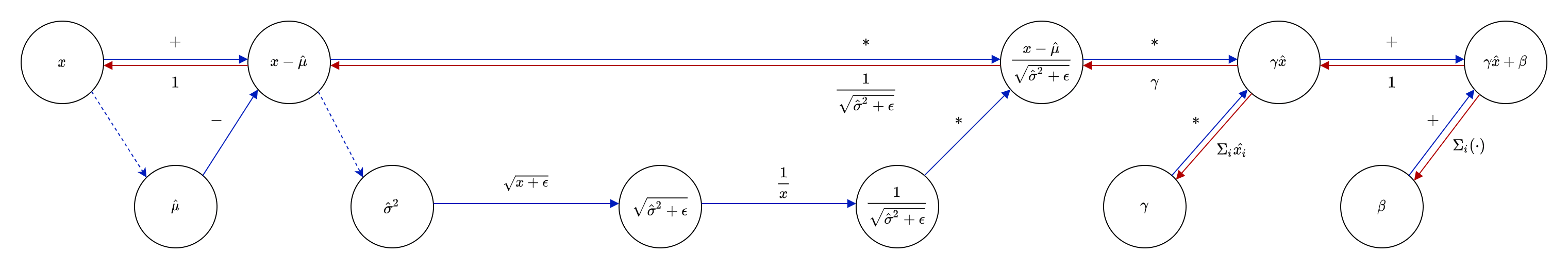
This seems like a reasonable attempt to fix the normalisation and results in reasonable performance, however, the performance is not the same as the original BatchNorm - and in some cases is worse than increasing epsilon above. Why is this? While the normalisation step is much the same, and thus the forward pass results in the same numbers, the backward pass is very different. Since the running statistics are detached from the batch statistics (there is no connection between them and thus they are treated as constants), the gradient is very different between BatchNorm and RunningBatchNorm. The gradient no longer takes into account the gradient of the batch statistics. And this effect turned out to be more important than normalising the internal layers2.
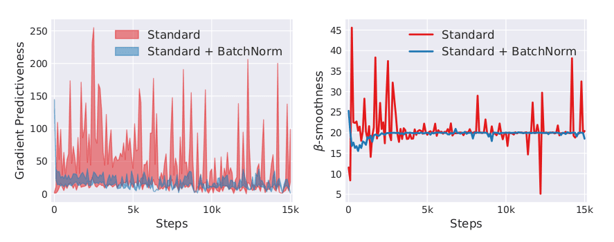
Comparing the Gradients
The original authors of BatchNorm left the "precise effect of Batch Normalization on gradient propagation" as a further area of study. So, after some time, the effect of BN on the loss landscape was studied2. It turns out that the whitening in BatchNorm using the batch statistics smooths the loss landscape. This means the gradients are more predictive - if you take a step in the direction of the current gradient, it is quite likely that you will continue moving in the same direction for the next gradient step. So if you doubled the learning rate, then things are just fine.
A smooth loss landscape prevents exploding and vanishing gradients and reduces the reliance on a good intialisation and a tuned, small learning rate. And while BatchNorm reparametrizes the loss using the batch statistics, it still keeps the same minima, since the parameters and can always be set to undo the whitening transform.
We can write out the gradients using backpropagation through a batchnorm layer and compare those with the RunningBN layer to see what changes.
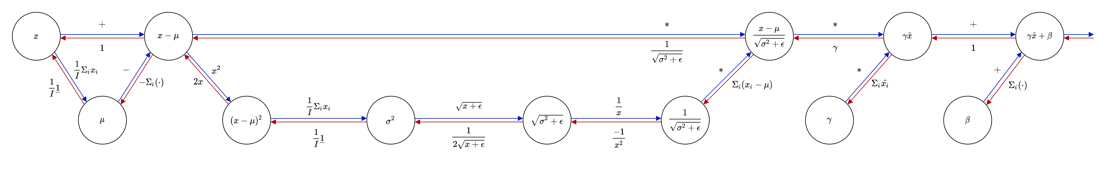
Backpropping through the BatchNorm layer attaches the gradients of the batch statistics to the gradient of the input. The simplified gradient of the output of BatchNorm with respect to the input thus looks like this:
The authors directly apply this expression to show that BatchNorm actually smooths the gradients, making training much easier. For further explanation on the properties of smoothness displayed by these gradients, see the extra note titled Lipschitz and Gradients, below. Comparing this to the RunningBN backprop graph, we can see that the statistics don't contribute to the gradient of the layer (except for the scaling by a constant - the running standard deviation).
Lipschitz
A lot of papers that explore the effects of BatchNorm and other adjustments to network architectures use something called Lipschitz continuity to describe the effect on smoothness of a function and thus help prove convergence for many gradient descent based algorithms. This gives us a mathematical framework to compare different architectures instead of looking at things empirically. But since it is a little extra math, it's just an aside.
A L-Lipschitz function is defined as follows:
This, in words, means the greatest change in the function is bounded by L. To take this further, the slope of the function between any 2 points is never greater than L. L, here, is called the Lipschitz constant. So this property is basically an upper estimate of the gradient of the function. Since we want stable gradients, a smaller L is preferred.
Beta smoothness is the exact same Lipschitz property, applied to the gradient of the function with a Lipschitz constant . -smoothness will thus bound the second derivative (the hessian) of the function. If the value is small it says that our gradients don't really change very much from place to place, while a large beta value says that the gradients are completely different if you move just a tiny bit from where you are now. So to make sure that our gradients don't change very much after consecutive gradient steps, we want a small value. This will enable us to take larger gradient descent steps (increase the learning rate) and feel more confident that our gradient is 'predictive' (that it actually is indicative of a good local minimum).
So to summarize, L-Lipschitz is a method of bounding the change in a function. To get good convergence with a first order method like gradient descent, we want the the -smoothness (-Lipschitz of ) to be small.
What does this mean for BatchNorm?
BatchNorm reduces the Lipschitz constant of the gradients of the loss, the -smoothness, making the loss landscape smoother, and more resilient to exploding/vanishing gradients, initialisations and learning rates2. As a result, the gradients are more predictive of finding a good minimum and thus we can increase the learning rate.
(BN also reduces the Lipschitz constant of the loss landscape, bounding the change in loss and making the gradients smaller and more stable, but this is almost a secondary effect to the beta smoothing.)
Since BN can undo the effects of the whitening using the parameters and , the method preconditions the optimisation - the optima remain the same but the landscape and the path that gradient descent takes to achieve an optimum are different.
A final word on eigenvalues
We've seen that the hessian is vital to optimisation convergence. If the eigenvalues of the hessian are all positive (a positive semi-definite hessian) then the function is convex (and at that point we can sit back and relax). While neural networks can be locally convex, they will not be globally convex due to non-linearities. By looking at the smallest (most negative) and largest eigenvalues of the hessian at different parts of the loss landscape, we can see how smooth the optimisation is and how close it is to convexity4. The Loss Landscape paper4 uses this technique to show how residual connections smooth the landscape, but we can also use it to see how BatchNorm changes it.
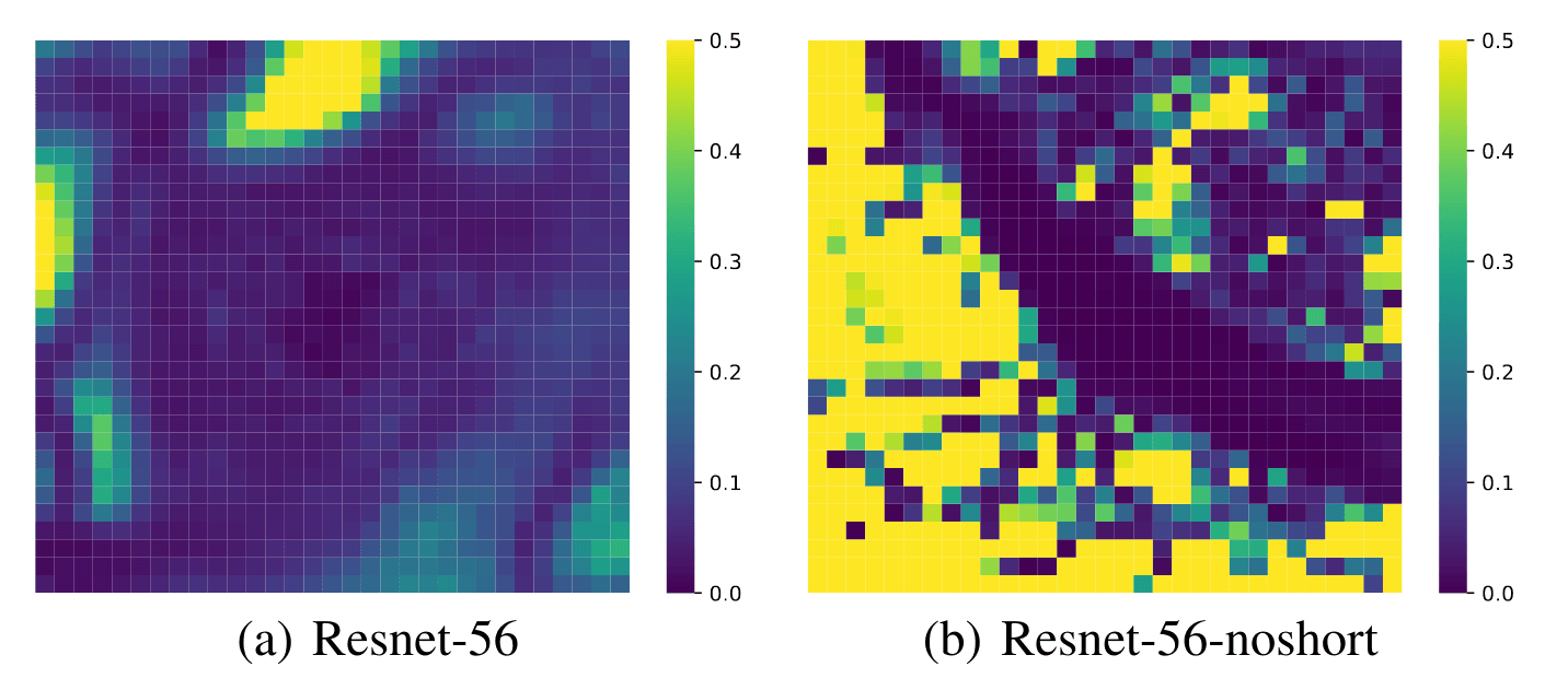
So if deep neural networks that don't have BN are more non-convex then they contain lots of ups and downs in the gradients, leading to vanishing or exploding gradients, and heavy reliance on good initialisation and learning rate tuning, to ensure they don't end up in some untrainable state. But with a much smoother landscape and gradients that "just get the job done" - they're not too big or small - the optimisation does not need to rely so heavily on initialisation and learning rate. In fact, an even larger learning rate will just get you there faster.
Alright, let's get back to it.
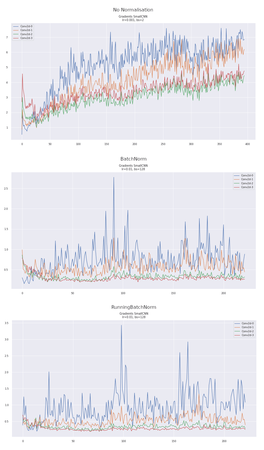
Empirical Gradients
As we saw above the gradients propagated through a BN layer and a Running BN layer differ significantly. But how does this show up in the gradients empirically, when training a network. Here we plot the L2 norm of the gradients throughout training for all the convolutional layers in the networks without and with BatchNorm and using RunningBatchNorm.
What we expect to see is how using BatchNorm results in gradients that don't explode or vanish. As we go deeper into the network, if the norm of the gradients keeps increasing or decreasing, then training becomes harder for the network. So ideally, we want to see the norms of the gradients remain roughly constant across iterations and layers. Additionally, we want fairly stable gradients that don't have any large drops or rises. In the non-normalised graph, we can see that there is a steep dropoff at the beginning, followed by a continual rise. The BatchNorm graph is much more stable. Furthermore, the L2 norm of the BN and RunningBN graphs are very similar, however, the L2 norm doesn't quite tell us enough about the quality of the gradients.
Where are BatchNorm's Improvements Coming From?
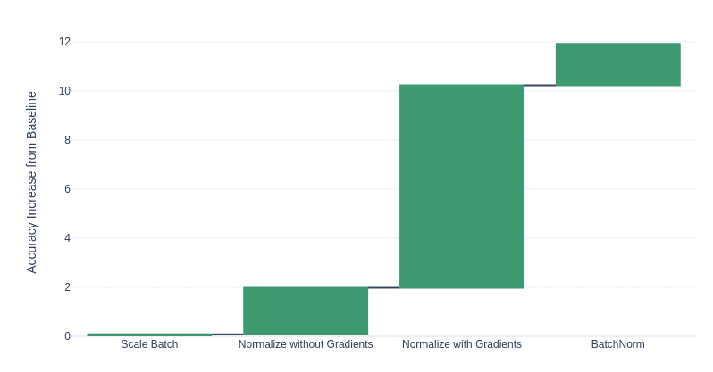
So if it's all about the gradients, then why are there other things in BN? The scaling and biasing, and the particular whitening (first and second moments)? Which parts of batchnorm cause the biggest improvements in the validation scores? We can separate BN into 2 parts: a normalisation step and a linear weighting step. The normalisation step uses the batch statistics to normalise across channels. We can also pull out the effect on the gradients by detaching the batch statistics from the normalisation step. By doing this, we can observe the effect of using the gradients in the backward pass. The linear weighting step multiplies each channel by a constant and adds a bias.
Here we compare the impact of each part of the BN algorithm on the validation loss and we can see that the effect of normalisation on the gradients is most important, yielding the majority improvement. The scaling and whitening themselves don't actually contribute too much to BN's performance. And this is why I particularly enjoy good ablation studies (such as the SqueezeExcite paper5), so that you know exactly where the improvements come from.
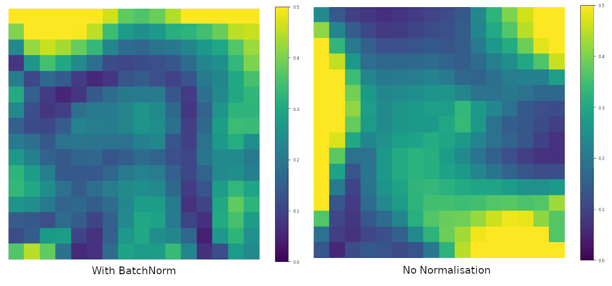
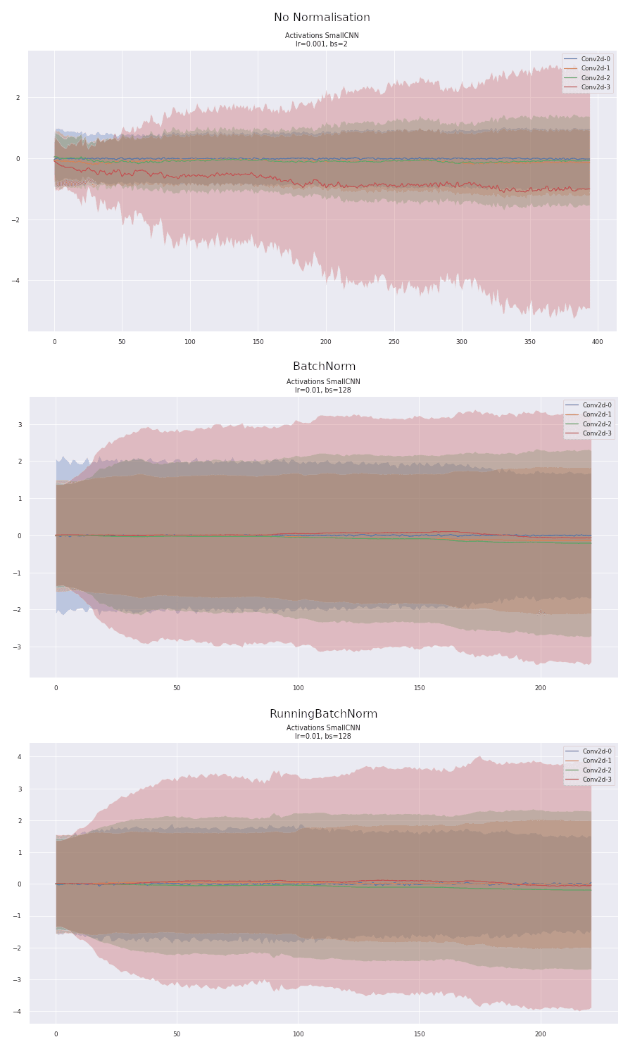
Comparing Activations
We can also compare the activations (the outputs) of the convolutional layers across normalisations. Similar to the original BN paper, we see that BN reduces the large variability in the activations and training seems to progress much smoother. What we want is a nice and stable training trajectory, without any large bumps that can kick us off the manifold of a good model that generalizes well. Without normalisation, the activations become biased with the last layer growing significantly and the others remaining small. The activations of the BatchNorm and RunningBN layers are very similar, showing how the forward pass remains essentially unchanged, despite BatchNorm performing better.
Other Normalisations
There have been several other attempts at creating a different normalisation layer to handle small batches which have mostly performed worse than BatchNorm except at the smallest batch sizes. Each attempt simply adjusts the dimensions over which to normalise.
LayerNorm6 normalises each layer individually, for every input. However, this prevents the network from learning to distinguish inputs that actually have a different distribution since each layer has the same normalised distribution.
In LayerNorm, if there are 2 images, with one image having a higher contrast than the other, then LayerNorm will normalize both images to the same level, preventing the network from learning anything based on the level of contrast. (This doesn't just apply to contrast but to any feature that occurs across layers.)
| bs | lr | Accuracy | Loss |
|---|---|---|---|
| 128 | 0.01 | 0.54 ± 0.02 | 1.43 ± 0.05 |
| 128 | 0.001 | 0.38 ± 0.02 | 1.81 ± 0.04 |
| 2 | 0.01 | 0.61 ± 0.01 | 1.22 ± 0.02 |
| 2 | 0.001 | 0.55 ± 0.00 | 1.38 ± 0.01 |
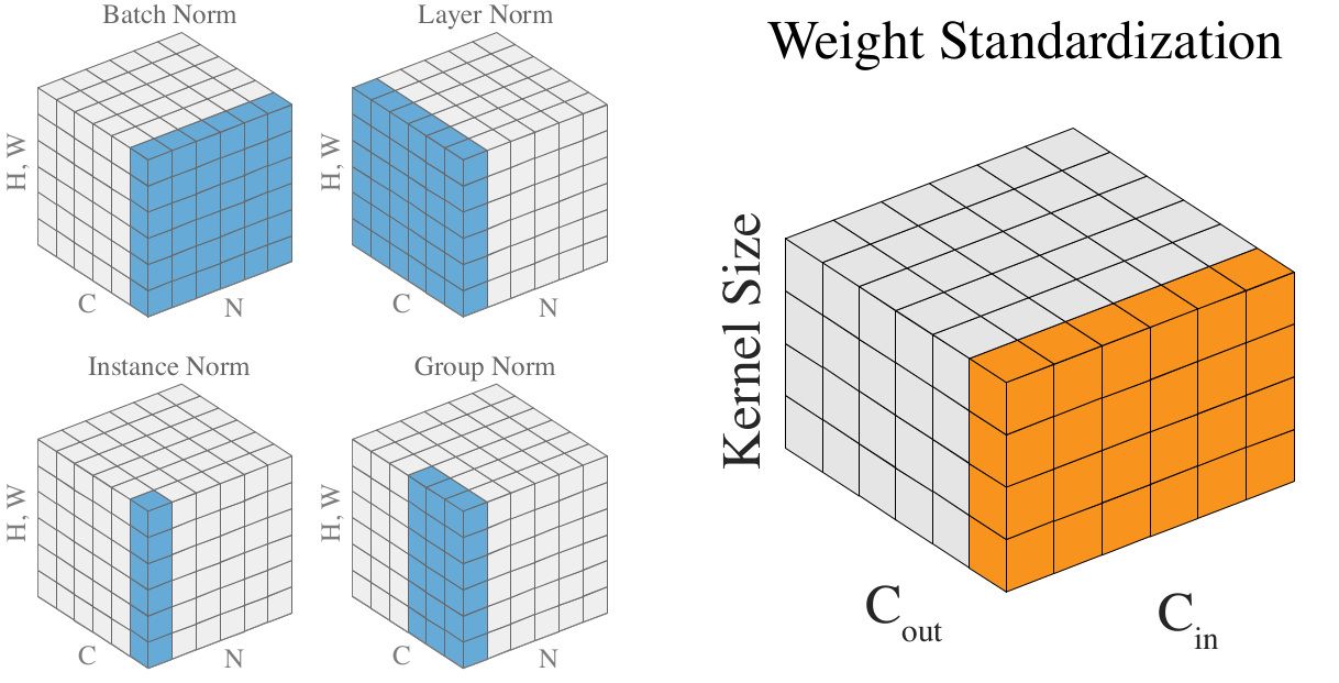
GroupNorm7 is a generalisation of LayerNorm. The method selects a number of groups for each normalisation to occur along the layer axis, ignoring batch information. At the one extreme is LayerNorm with a single group across the entire layer, and at the other extreme is a group for every channel, called InstanceNorm (which is typically only used for style transfer). However, GroupNorm allows different numbers of groups and each group is normalized, allowing the network to compensate for a lack of batch information, by grouping channels (more on this below).
| bs | lr | Accuracy | Loss |
|---|---|---|---|
| 128 | 0.01 | 0.57 ± 0.01 | 1.32 ± 0.01 |
| 128 | 0.001 | 0.40 ± 0.00 | 1.76 ± 0.02 |
| 2 | 0.01 | 0.62 ± 0.01 | 1.19 ± 0.02 |
| 2 | 0.001 | 0.59 ± 0.01 | 1.27 ± 0.02 |
So while these methods include the gradients of the sample statistics at least across some dimensions, they do not include batch information, and often perform worse than BatchNorm unless the batch size is small.
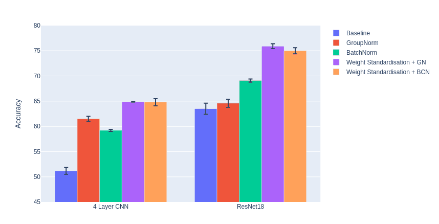
Weight Standardisation and Batch-Channel Normalisation
So BatchNorm smooths the loss landscape which results in a bunch of nice properties: faster training, larger learning rates, better generalisation, less reliance on good initialisation. All of these properties are because of the effect of the normalization using the batch statistics on the gradient. Now that this is known, could we adjust the normalization so that the gradient has the same smoothing without the normalization across activation batches. The Weight Standardisation paper3 points out that the activations are simply one step removed from the weights of the network and the weights are what actually receive the gradient. So instead, we can standardise the weights instead of the activations, and achieve the same smoothing effect (a reduction in Lipschitz constant, which is proved in the paper, in a similar manner to the way it's proved for BatchNorm).
Now you may notice, that if the weights are standardised, then the activations after our convolution will be huge. So the authors assume the use of an activation normalization scheme like GN after this to shift the activations to a regular place once more. The effects of this, they claim, are additive on the smoothness of the landscape.
The WS paper also notices another property that comes as a corollary to BatchNorm: it avoids parts of the network where neurons are completely zero and have no gradient (such as the negative half after a ReLU activation) and are thus eliminated from training. The authors call this an "elimination singularity"3:
Elimination singularities refer to the points along the training trajectory where neurons in the networks get eliminated. Eliminable neurons waste computations and decrease the effective model complexity. Getting closer to them will harm the training speed and the final performances. By forcing each neuron to have zero mean and unit variance, BN keeps the networks at far distances from elimination singularities caused by non-linear activation functions.
BatchNorm reduces elimination singularities (in ReLU based networks) by ensuring that at least some of the activations of each channel/neuron in a layer are positive and receive a gradient. It also ensures that each channel isn't underrepresented since they are normalized across the batch for each channel. Channel based methods (GN, LN) normalize the same across channels, resulting in some channels having more negative values which will be eliminated and other channels which are underrepresented. GroupNorm, however, somewhat helps this problem as each group will have some positive neurons that aren't eliminated.
So without access to batch information, we come closer to elimination singularities, but in practice, collecting batch information is fairly easy - just use running BatchNorm like above. So we can combine batch info with GN by adding in RunningBN (which the authors call Batch Channel Norm) which typically results in even better performance.
| bs | lr | Accuracy | Loss |
|---|---|---|---|
| 128 | 0.01 | 0.59 ± 0.00 | 1.26 ± 0.01 |
| 128 | 0.001 | 0.39 ± 0.01 | 1.76 ± 0.00 |
| 2 | 0.01 | 0.65 ± 0.00 | 1.08 ± 0.01 |
| 2 | 0.001 | 0.58 ± 0.01 | 1.27 ± 0.03 |
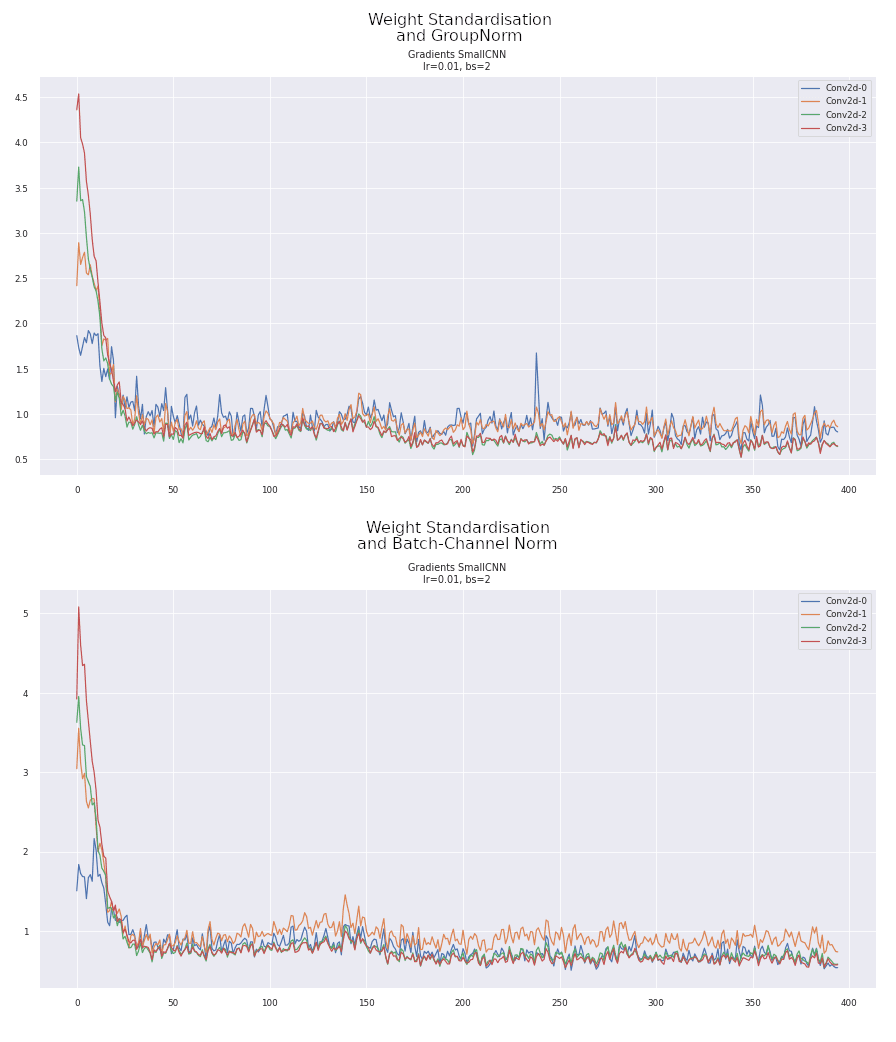
Weight Standardisation Gradients
Comparing the gradients of WS with GN and BCN shows an interesting peak at the start of training. I don't have a good explanation as to its presence but I don't think it is particularly good for training. Nevertheless, the gradients thereafter are particularly stable, remaining around 1 throughout with fewer spikes than BatchNorm.
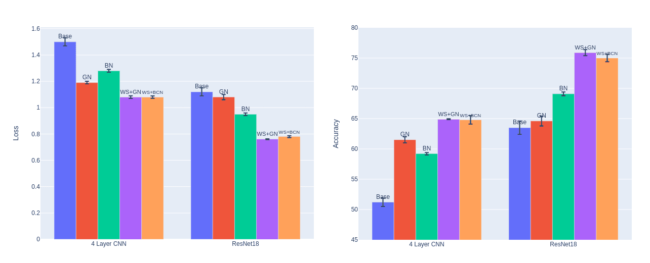
Conclusion
BatchNorm owes most of its success to the effect it has on the gradients. By smoothing the loss landscape and making the gradients more stable, BatchNorm doesn't need to rely so heavily on good initialisation and learning rate tuning to avoid vanishing or exploding gradients. By considering how the gradients are affected by BatchNorm, we can create a new layer to perform equally to BatchNorm without the constraint on batch size. By applying the standardisation to the weights instead of activations, we can achieve the same effect on the gradients. Additionally, changing to weight standardisation often leads to improved network performance.
Limitations
- Training was fairly short (only 3 epochs) so we don't see how things progress further on.
- Only did 3 runs per test although results are fairly stable.
- There are other methods that can take the place of normalization that I have not mentioned here. For example, SELU8, Fixup9, and network deconvolution10.
- For all the experiments, I ignored wall time, which is approximately 5x longer for the small batch networks.
Feedback
If you're still reading and if you enjoyed the article (or didn't), please feel free to send me a note about what you liked and what you didn't. I'd love to improve and your feedback means a lot! See about page for contact.
References
Footnotes
-
Batch Normalization: Accelerating Deep Network Training by Reducing Internal Covariate Shift arxiv ↩
-
How Does Batch Normalization Help Optimization? arxiv ↩ ↩2 ↩3 ↩4 ↩5
-
Micro-Batch Training with Batch-ChannelNormalization and Weight Standardization arxiv ↩ ↩2 ↩3
-
Fixup Initialization: Residual Learning Without Normalization arxiv ↩