From MobileNet to EfficientNet

In this article, I'm going to walk through the architectural implementations that led from the first MobileNet architecture to the state of the art EfficientNet architecture, with a bunch of improvements in between. The MobileNet architecture was aimed at reducing the computational requirements for large neural networks without a large drop in performance on the classification task. This was with the particular goal of deploying the networks on edge devices, like mobile phones. After several years of iterating on the same design ideas, EfficientNet was built using the same building blocks to create a high performance, low cost network.

MobileNetV1

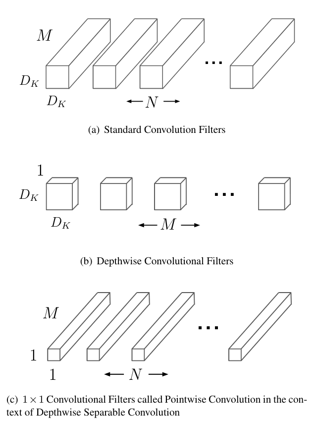
The basic building block for most of the successes in image recognition and processing due to deep learning comes from using many convolutional layers¹. These layers capture features present in the input images and build up complexity in the representations, the deeper into the network you go². In the MobileNet paper³, the aim was to reduce the computational complexity required by each convolutional layer. To do this, they designed a new "separable" convolution layer, where the convolution operation would be separated into 2 parts. The first part would apply the kernel operation to each channel individually, as opposed to doing it for all the channels. This part would capture features of the input but with far fewer parameters. This is called a depthwise convolution since the convolution happens independently for every channel along the depth axis.

The second part would then apply a convolution with a kernel size of 1 so that the newly created channel features could be combined. This is called a pointwise convolution due to the 1x1 kernel size. Additionally, the 1x1 kernel could be used to change the number of channels in the output.

Top: Regular convolution applied the kernel to all of the channels. Middle: Depthwise convolution applies each kernel to a single input channel. Bottom: Pointwise convolution applies a 1x1 kernel size to the output of the depthwise convolution to create combinations of each of the different features.

The authors of the paper then stacked a bunch of these layers together to build the first MobileNet. They added 2 additional scaling parameters on top of this base network that you could tune to select between greater accuracy and lower computational cost. The first was model width which is a scalar multiplier for all the number of channels in the network. The second is the input resolution, an implicit parameter which is chosen when you process the images into the desired height and width.

The network achieved similar accuracy on ImageNet as an equivalent regular CNN but at around 15% of the computational cost. Below is a short snippet of code implementing the critical layers in PyTorch.

# To apply a depthwise convolution in pytorch, the
# groups parameter is set to the number of channels.
class DepthWiseConv2d(nn.Conv2d):
  "Depth-wise convolution operation"
  def __init__(self, channels, ks=3, st=1):
    super().__init__(channels, channels, ks, stride=st,
                     padding=ks//2, groups=channels)

# A pointwise convolution has a 1x1 kernel size.
class PointWiseConv2d(nn.Conv2d):
  "Point-wise (1x1) convolution operation."
  def __init__(self, cin, cout):
    super().__init__(cin, cout, 1, stride=1)

# The mobilenet building block consists of a
# depthwise conv, batchnorm, relu, pointwise
# conv, batchnorm and relu again. These blocks
# are simply combined into the full mobilenet
# architecture. See Table 1 in the paper.
class MobileNetConv(nn.Module):
  "The MobileNetV1 convolutional layer"
  def __init__(self, cin, cout, ks=3, st=1,
               act=nn.ReLU(True)):
    super().__init__()
    self.dwconv = DepthWiseConv2d(cin, ks=ks, st=st)
    self.bn1 = nn.BatchNorm2d(cin)
    self.act = act
    self.pwconv = PointWiseConv2d(cin, cout)
    self.bn2 = nn.BatchNorm2d(cout)

  def forward(self, x):
    x = self.act(self.bn1(self.dwconv(x)))
    x = self.act(self.bn2(self.pwconv(x)))
    return x

MobileNetV2

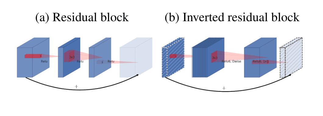
A short while later, the second version of MobileNet was released. Before this, the ResNet⁴ architecture had proven particularly accurate at ImageNet and thus MobileNetV2 incorporated the idea of residual blocks into the depthwise separable convolution layer they created. The residual network simply adds an identity path around each of the convolutional layers and adds the output of the convolutional block to the identity path. This allows the network to learn the difference from the identity and allows gradients the propagate better.

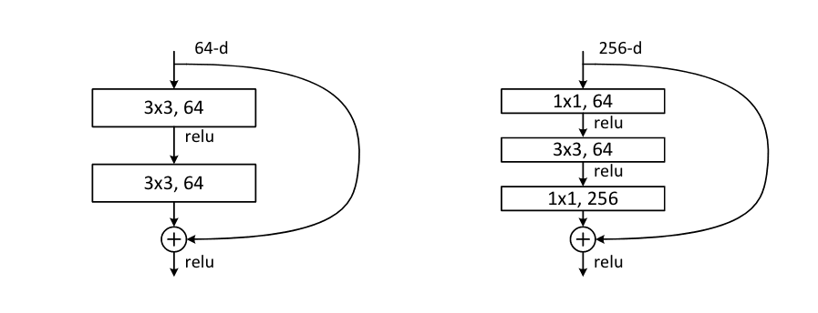
Furthermore, for large residual networks, a "bottleneck" layer is used to contract the number of channels using a 1x1 convolution, apply a computationally expensive 3x3 convolution on the reduced channel number and then expand the number of channels with another 1x1 convolution.

Left: The normal residual block. Right: the bottleneck residual block.

MobileNetV2⁵ uses the same depthwise separable convolution as v1 but applies a residual connection around the block. Furthermore, instead of contracting the number of channels to save computation, the network expands the input number of channels using a pointwise convolution, followed by the depthwise convolution that operates at a reduced computational complexity and then the channels can be contracted again so that they can be added to the input residual path. This layer is called the inverted residual block and is the main building block of MobileNetV2.

Left: the residual bottleneck which reduces the number of channels before the 3x3 convolution in the middle. Right: An inverted residual block expands the number of channels, then applies a depthwise convolution, and then contracts the number of channels back to the original size so that it can be added to the identity path.

The MobileNetv2 paper also does not place any non-linearity after the pointwise expansion convolution. The authors state that these non-linearities destroy information and that a linear layer is the same as the non-linear counterpart if the input lies on a lower dimensional manifold. See the paper for more details. Finally, a ReLU6 non-linearity is used due to it's robustness with low precision computation.

Below is an implementation of the inverted residual block.

class InvertedResidualBlock(nn.Module):
  """
  Inverted residual block from mobilenetv2.
  For strides>1 or cin!=cout, the input does
  not get added to the residual.
  """
  def __init__(self, cin, cout, stride=1,
              expansion_ratio=6, act=nn.ReLU6(True)):
    super().__init__()
    self.stride = stride
    self.same_c = cin == cout
    self.block = nn.Sequential(
        PointWiseConv2d(cin, cin*expansion_ratio),
        nn.BatchNorm2d(cin*expansion_ratio),
        act,
        DepthWiseConv2d(cin*expansion_ratio, st=stride),
        nn.BatchNorm2d(cin*expansion_ratio),
        act,
        PointWiseConv2d(cin*expansion_ratio, cout),
        nn.BatchNorm2d(cout),
    )

  def forward(self, x):
    residual = self.block(x)
    if self.stride != 1 or not self.same_c:
        return residual
    else:
        return x + residual

SENet

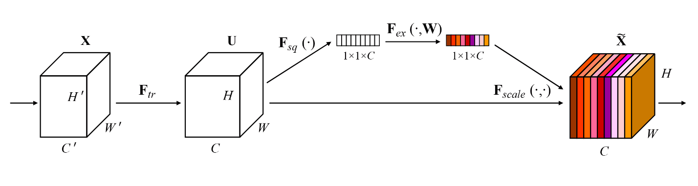
The squeeze and excitation network (SENet)⁶ adds another building block to the basic ResNet (and other architectures). The squeeze and excitation module takes the input, applies global pooling, then goes through a fully connected, ReLU, fully connected layer which is then sigmoided and multiplied across the channels of the original input. The idea behind this block is similar to that of attention where the network can learn to capture interactions across channels. Each channel gets globally aggregated information from all of the other channels. The paper's ablation study is particularly good and is certainly worth the read.

The first linear layer contracts the SE branch by a specified reduction_ratio, set to 16. This reduces the computation in the block and allows the layer to capture non-linear interactions between channels before expanding back to the original number of channels.

The squeeze and excitation block multiplies all of the output channels by an aggregated input to capture channel-wise feature interactions.

A modified version of the architecture won the ILSVRC 2017 challenge. The main SE block is implemented below and is usually slotted into residual layers before the identity path is added with the residual. Several other configurations are explored in the ablation.

class SqueezeExcite(nn.Module):
  "Squeeze and excitation module."
  def __init__(self, cin, reduction_ratio=16):
    super().__init__()
    self.squeeze = nn.Sequential(
        nn.AdaptiveAvgPool2d(1),
        nn.Conv2d(cin, cin//reduction_ratio, 1),
        nn.ReLU(True),
        nn.Conv2d(cin//reduction_ratio, cin, 1),
        nn.Sigmoid()
    )

  def forward(self, x):
    squeeze = self.squeeze(x)
    return x * squeeze

MobileNetV3

MobileNetV3⁷ simply takes the building blocks of v2, and adds a few tricks. First, they add the squeeze and excitation module after the depthwise convolution with a smaller reduction ratio of 4. They initially use the swish⁸ non-linearity which is calculated by $y = x σ (x)$ where $σ$ is the sigmoid function. This activation tends to improve results by around 1%. Nevertheless, due to the computational complexity of the non-linearity, they opt to adapt the function to a hard version of the original by using a piecewise linear approximation. To find a good baseline network, the authors run neural architecture search (NAS) on larger blocks initially and, after this, on the individual layers within the blocks. This search generates a low latency, high accuracy baseline that can then be scaled using the same width and resolution scaling seen in MobileNetV1 and MobileNetV2. Additionally, the authors find a large and a small model in the architecture search.

class HardSwish(nn.Module):
  def forward(self, x):
    return x*(F.relu6(x+3)/6)

class InvertedResidualV3(nn.Module):
  """
  MobileNetV3 inverted residual block with squeeze
  excite block embedded into residual layer, after the
  depthwise conv. Uses the HardSwish activation.
  """
  def __init__(self, cin, cout, ks=3, stride=1,
              expansion_ratio=4, squeeze_ratio=None,
              act=HardSwish()):
    super().__init__()
    self.stride = stride
    self.same_c = cin == cout
    self.exp = round(cin*expansion_ratio)
    self.block = nn.Sequential(
        PointWiseConv2d(cin, self.exp),
        nn.BatchNorm2d(self.exp),
        act,
        DepthWiseConv2d(self.exp, st=stride),
        nn.BatchNorm2d(self.exp),
        act,
        SqueezeExcite(self.exp,
                      reduction_ratio=squeeze_ratio),
        PointWiseConv2d(self.exp, cout),
        nn.BatchNorm2d(cout),
    )

  def forward(self, x):
    residual = self.block(x)
    if self.stride != 1 or not self.same_c:
        return residual
    else:
        return x + residual

EfficientNet

Finally, the EfficientNet paper⁹, which came out at nearly the same time as the MobileNetV3 paper and has several intersecting authors uses several similar ideas to the MobileNetV3 paper. They too add the SE block and use the swish activation, however, the EfficientNet paper examines scaling of neural networks. They find that the best gains come from scaling the width, resolution (like the mobilenets) and depth of the network simultaneously.

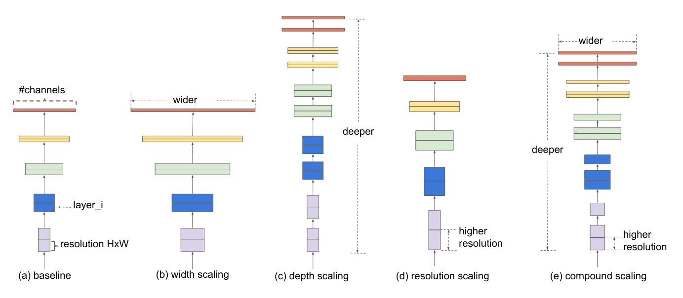
To achieve this, they start by using NAS to find a small baseline model. They then scale the baseline according to the equation below. The constants $α$ , $β$ and $γ$ are determined by a small grid search done on the baseline model. The whole point of this search and scale technique being to find a good model but without needing to use a lot of computational power searching over a large model.

d e pt h = α^{ϕ} w i d t h = β^{ϕ} reso l u t i o n = γ^{ϕ} s . t . α \times β^{2} \times γ^{2} \approx 2 α \geq 1, β \geq 1, γ \geq 1

Once these values are found, the baseline EfficientNet-B0 is scaled up with $ϕ$ . This leads to EfficientNet-B1 through B8.

The EfficientNet paper also includes a bunch of tricks in training like stochastic depth, auto-augment, drop-connect, and increasing dropout, but they don't particularly say whether the additions improve things and by how much. The paper lacks a comprehensive ablation study to root out the biggest improvements to the network. Several reimplementors have had difficulty reimplementing the paper and achieving the same levels of performance.

Nevertheless, the authors have continued improving the network and getting better results by adding adversarial training¹⁰ into the mix and using network distillation in a technique called "noisy student"¹¹ which improves the state of the art on ImageNet even more.

And that is a whirlwind tour up to the current state of the art in ImageNet classification. Thanks for reading!

References

ImageNet Classification with Deep Convolutional Neural Networks link ↩
Visualizing and Understanding Convolutional Networks arxiv ↩
MobileNets: Efficient Convolutional Neural Networks for Mobile Vision Applications arxiv ↩
Deep Residual Learning for Image Recognition arxiv ↩
MobileNetV2: Inverted Residuals and Linear Bottlenecks arxiv ↩
Squeeze-and-Excitation Networks arxiv ↩
Searching for MobileNetV3 arxiv ↩
Searching for Activation Functions arxiv ↩
EfficientNet: Rethinking Model Scaling for Convolutional Neural Networks arxiv ↩
Adversarial Examples Improve Image Recognition arxiv ↩
Self-training with Noisy Student improves ImageNet classification arxiv ↩

Tom Tumiel